utu.dem.plowman#
- utu.dem.plowman(intensity, uncertainty, response, axis_channel, axis_temperature, smoothness=8, chi2_target=1, tolerance=0.1, steps=(0.1, 0.5), iterations_max=100, iterations_min=5, floor=None)[source]#
Invert intensities for a differential emission measure (DEM), the way Plowman & Caspi (2020) do.
The DEM is piecewise linear in \(\log_{10} T\) between the temperatures of
response, and is found as the exponential of a piecewise linear function, which makes it positive everywhere without a constraint. The fit is regularized by the square of the derivative of the logarithm of the DEM, which penalizes changes of more than aboutsmoothnesse-foldings per decade of temperature, and is stopped once the reduced \(\chi^2\) reacheschi2_targetrather than driven below it.Each pixel is independent, and they are inverted in parallel by a compiled kernel which reproduces the reference implementation to rounding error. See the notes below.
If
intensity,uncertainty, or the outputs ofresponseare uncertain, so are the DEM and \(\chi^2\): their nominal values are those of the nominal inputs, and each sample of the distribution is inverted as one more pixel.- Parameters:
intensity (Quantity | AbstractScalar) – The observed intensity in each channel. Every axis other than
axis_channelis a separate inversion.uncertainty (Quantity | AbstractScalar) – The one-sigma uncertainty of
intensity, in the same units.response (FunctionArray[AbstractScalar, AbstractScalar]) – The temperature response of each channel: its inputs are the temperatures along
axis_temperature, increasing and with units of temperature, and its outputs are the responses alongaxis_temperatureandaxis_channel, in units ofintensityper unit emission measure. The channels must be in the same order as those ofintensity.axis_channel (str) – The name of the axis along the channels of
intensityandresponse.axis_temperature (str) – The name of the axis along the temperatures of
response.smoothness (float) – The number of e-foldings per decade of temperature which the DEM may change by before the regularization starts to resist, called \(\delta_0\) (and
drv_con) in the paper. Smaller is smoother. The paper finds that anything from 4 to 16 fits AIA data.chi2_target (float) – The reduced \(\chi^2\) the iteration aims for.
tolerance (float) – How close to
chi2_targetis close enough, and how little improvement per unit step counts as having stalled.steps (tuple[float, float]) – The small and the large fraction of the way to the linearized solution to try at each step. The step taken is interpolated between them to land on
chi2_target.iterations_max (int) – The most steps to take for any one pixel.
iterations_min (int) – The number of steps to take before giving up on a pixel whose \(\chi^2\) has stalled.
floor (Quantity | float | None) – The least intensity the initial guess assumes in any channel, which must be positive and in units convertible to those of
intensity. It changes the result only for pixels with almost no signal, and only through where the iteration starts. IfNone, it is 0.01 in the units ofintensity, as in the reference.
- Returns:
dem – The DEM at each temperature of
response, per unit \(\log_{10} T\), in units ofintensityover the units of the outputs ofresponse: \(\mathrm{cm^{-5}}\) for responses in \(\mathrm{DN\,cm^5\,s^{-1}}\) and intensities in \(\mathrm{DN\,s^{-1}}\).chi2 – The reduced \(\chi^2\) of each pixel, or \(-1\) where the first step failed, in which case the DEM is NaN. A NaN or non-positive uncertainty fails a pixel this way.
- Return type:
tuple[FunctionArray[AbstractScalar, AbstractScalar], AbstractScalar]
Notes
This is
simple_reg_demfrom the appendix of Plowman & Caspi (2020), as distributed in EMToolKit. Its defaults are those of the code listing in that appendix, which are not the ones its text describes: the text gives 15 initial steps, steps of 0.1 and 0.75, a smoothness of 4, and a tolerance of \(10^{-4}\), and describes choosing whichever of the two trial steps has the lower \(\chi^2\), whereas the code interpolates between them. The code is what produced the published results, and what is reproduced here.Against the reference, the DEMs agree to about \(10^{-11}\) relative on AIA data and on the random test DEMs of the paper. They do not agree to the last bit, and cannot: the regularization matrix is singular on its own (it does not penalize a constant), and where the data say little the linear systems are close to it, so the rounding errors of any two implementations of the Cholesky factorization grow by orders of magnitude over the iteration. A port of the reference with
numpy.linalgin place ofscipy.linalgdisagrees with it by as much. The worst cases are pixels with no signal, at about \(10^{-6}\), and pixels the model cannot fit at all, whose \(\chi^2\) stays far above the target and whose DEM is meaningless in either implementation.Negative intensities are set to zero before the fit, as in the reference. The initial guess is the flat DEM which best fits the intensities, each raised to at least
floor. In the reference, the floor is a bare 0.01 in whatever units the data are in, which is the default here too, but it can be given in any units. The reference takes a negative uncertainty as positive, where this fails the pixel.The kernel takes about 20 to 30 microseconds per pixel on one core, some 40 times faster than the reference, and runs on every core: a whole AIA image of \(4096^2\) pixels takes about 12 seconds on 24 cores, against about four hours for the reference. The first call compiles the kernel, which takes a few seconds, and caches it to disk for later sessions.
Examples
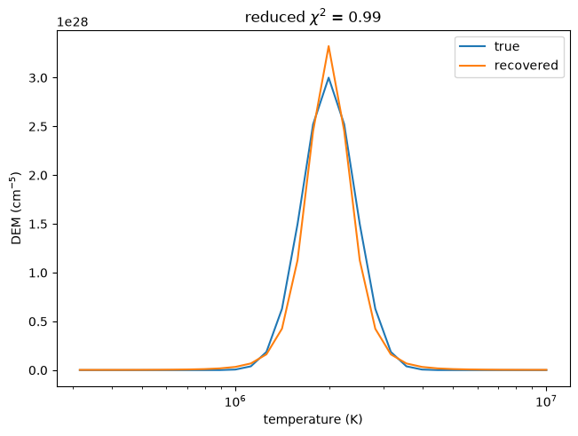
Six channels whose responses peak at different temperatures, observing a plasma whose DEM peaks near 2 MK, with the uncertainty of a second of photon counting, and the DEM recovered from them.
import astropy.units as u
import matplotlib.pyplot as plt
import named_arrays as na
import numpy as np
import utu

temperature = 10 ** na.linspace(5.5, 7, axis="temperature", num=31) * u.K
logt = np.log10(temperature.value)

# Gaussian responses in log T, one per channel
peak = na.linspace(5.7, 6.9, axis="channel", num=6)
response = na.FunctionArray(
    inputs=temperature,
    outputs=1e-25 * np.exp(-(((logt - peak) / 0.15) ** 2)) * u.DN * u.cm**5 / u.s,
)

# the true DEM, and the intensities it would produce
dem_true = 3e28 * np.exp(-(((logt - 6.3) / 0.12) ** 2)) / u.cm**5
intensity = (response.outputs * dem_true).sum("temperature") * 0.05
uncertainty = np.sqrt(intensity * u.DN / u.s) + 1 * u.DN / u.s

dem, chi2 = utu.dem.plowman(
    intensity=intensity,
    uncertainty=uncertainty,
    response=response,
    axis_channel="channel",
    axis_temperature="temperature",
)

fig, ax = plt.subplots(constrained_layout=True)
na.plt.plot(temperature, dem_true, ax=ax, axis="temperature", label="true")
na.plt.plot(dem.inputs, dem.outputs, ax=ax, axis="temperature", label="recovered")
ax.set_xscale("log")
ax.set_xlabel(f"temperature ({temperature.unit:latex_inline})")
ax.set_ylabel(f"DEM ({dem.outputs.unit:latex_inline})")
ax.set_title(f"reduced $\\chi^2$ = {chi2.ndarray:.2f}")
ax.legend();